This topic is essentially a continuation of topic 3, looking at inheritance of two traits instead of just one. It was actually a very fun topic which I enjoyed a lot. In the start it seemed very easy, but it turned out to be a little hard after all. I would highly recommend going back and revise topic 3 if something is unclear. The most challenging concept in this topic is probably linked genes. I will refer to some good videos at the bottom of the page as usual. Otherwise, the best strategy for this chapter is probably to do a lot of exercises because I bet that there are a lot of marks to get for this topic on the exams.
Points for revision:
- Mendelian genetics with one trait
- Mendelian genetics with two traits
- Isolation, selection, and speciation
Meiosis
Meiosis or reduction division is the process of turning one diploid cell (2n) into four haploid cells (n). Meiosis is incredibly important because the various processes increase the genetic variation of offspring. The process of meiosis is covered in topic 3, so I will go more into the effects of the processes in this topic.

Recombination
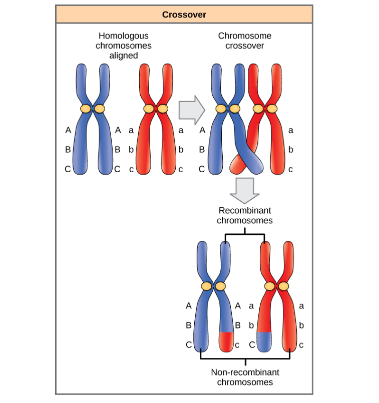
As you may recall, meiosis happens in two stages, meiosis 1 and meiosis 2. Meiosis 2 is essentially the same as mitosis, but meiosis 1 is special. The first step in meiosis 1 that makes it special is recombination during prophase 1. In prophase 1, the homologous chromosomes gather into 23 pairs called bivalent chromosomes, and sometimes, these bivalent chromosomes may overlap. When this happens, recombination occurs. Recombination is when two non-sister chromatids overlap and exchange genetic information. This means that the chromosome from the dad can change genes with the chromosome from the mom. Recombination can be visualized as cutting the two chromosomes at the same place (the location of the cut is called the chiasmata). After the cut, the cut off DNA segments are swapped and glued to the other chromosome again. Recombination means that new alleles may be created. For example, if the chromosome from the dad has two genes each with one allele A and B, and the mom has the same genes but with alleles a and b. Without recombination, the only possible formation of gametes would be AB and ab, but with recombination, it is now possible to form Ab and aB, in addition to AB and ab. The new genotypes produces by recombination (Ab and aB), are called recombinants. This will be important for dihybrid crosses, which we will come back to later.
Random orientation
The other step which is special for meiosis is random orientation in metaphase 1 and 2. In metaphase 1, the homologous chromosome pairs group together down two lines of the cell. These homologous chromosomes are called bivalent chromosomes, and one chromosome of the bivalent pair is on one side of the division, while the other one is on the other side (I will call the sides the left and right side for ease). This means that for a bivalent pair, a chromosome can either be on the left or right side. The chromosomes may be interchanged because of random orientation. Random orientation means that it is random which of the chromosomes are on which side of the divide. Let us try to visualize it with only one bivalent chromosome. We have two chromosomes and two sides they can be on; it is almost like a coin. A coin has two faces (representing the two chromosomes), and two sides the coin can face (up or down, in this case representing left and right). When we flip the coin, we have a 50/50 percent chance of a side facing up or down. It is the same with bivalent chromosomes. Random orientation is basically flipping the coin, but in humans there are 23 coins because of the 23 chromosomes. All the coins are flipped independently, and therefore for each coin there are 2 possibilities, so for 23 coins there are 2 x 2 x 2 x… x 2, 23 times, or 2^23. This gives more than 8 million combinations, just due to random orientation. This happens the same way in metaphase 2, but in this case, it is not bivalent chromosomes, but sister chromatids. If meiosis is unclear, go back and revise topic 3.
Crossing over and random orientation means that meiosis can create a lot of variation, in addition to creating genotypes that were not present at all in the parent genome.
Mendelian genetics with one trait
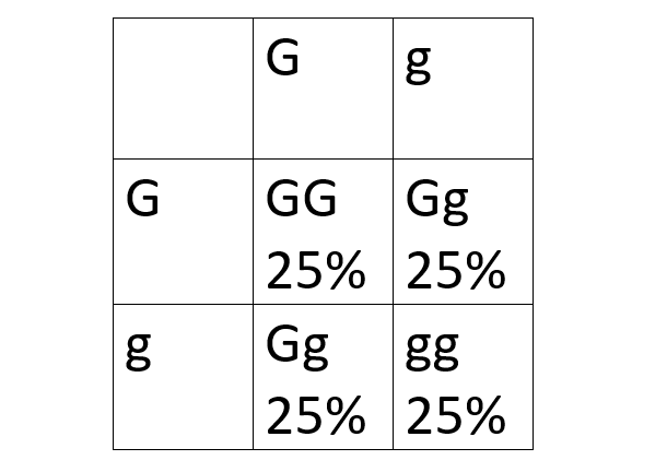
Gregor Mendel experimented with pea plants, and what he found was that even though particles of inheritance could be combined in a pea plant, they were inherited independently. We now know that the particles of inheritance are of course chromosomes and that “inherited independently” is a result of the chromosomes splitting up during meiosis. Mendel’s theory (now called Mendel’s first law) works perfectly well with one trait controlled by one gene only because one gene can only be on one location on one chromosome. This means that if a mom has an allele G from her mom, and an allele g from her dad, the gamete (egg) has a 50% chance to carry either G or g. This is the same for the gamete (sperm) from the dad if he got the same alleles from his parents. The resulting combinations can be visualized in the very familiar two by two Punnett square. The gametes formed during meiosis has equal probability of containing either of the two alleles.
Another pattern Mendel found was that traits were inherited independently of each other. This is Mendel’s second law, or the law of independent assortment. This also works perfectly fine with one gene controlling one trait for the same reason as the first law. However, it gets interesting when two or more traits are added to the equation.
Mendel’s first and second law are essentially saying the same, the genotypes of the offspring have the same probability of being formed because the gametes have the same probability of being formed. This is basically to say that each square in a two by two Punnett square has a 25% chance of being the genotype of the offspring.
Mendelian genetics with two traits
To see how to make dihybrid Punnett squares, watch this video:
https://www.youtube.com/watch?v=Y1PCwxUDTl8
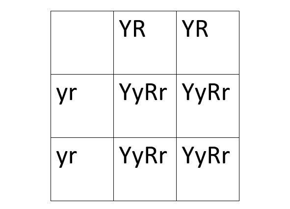
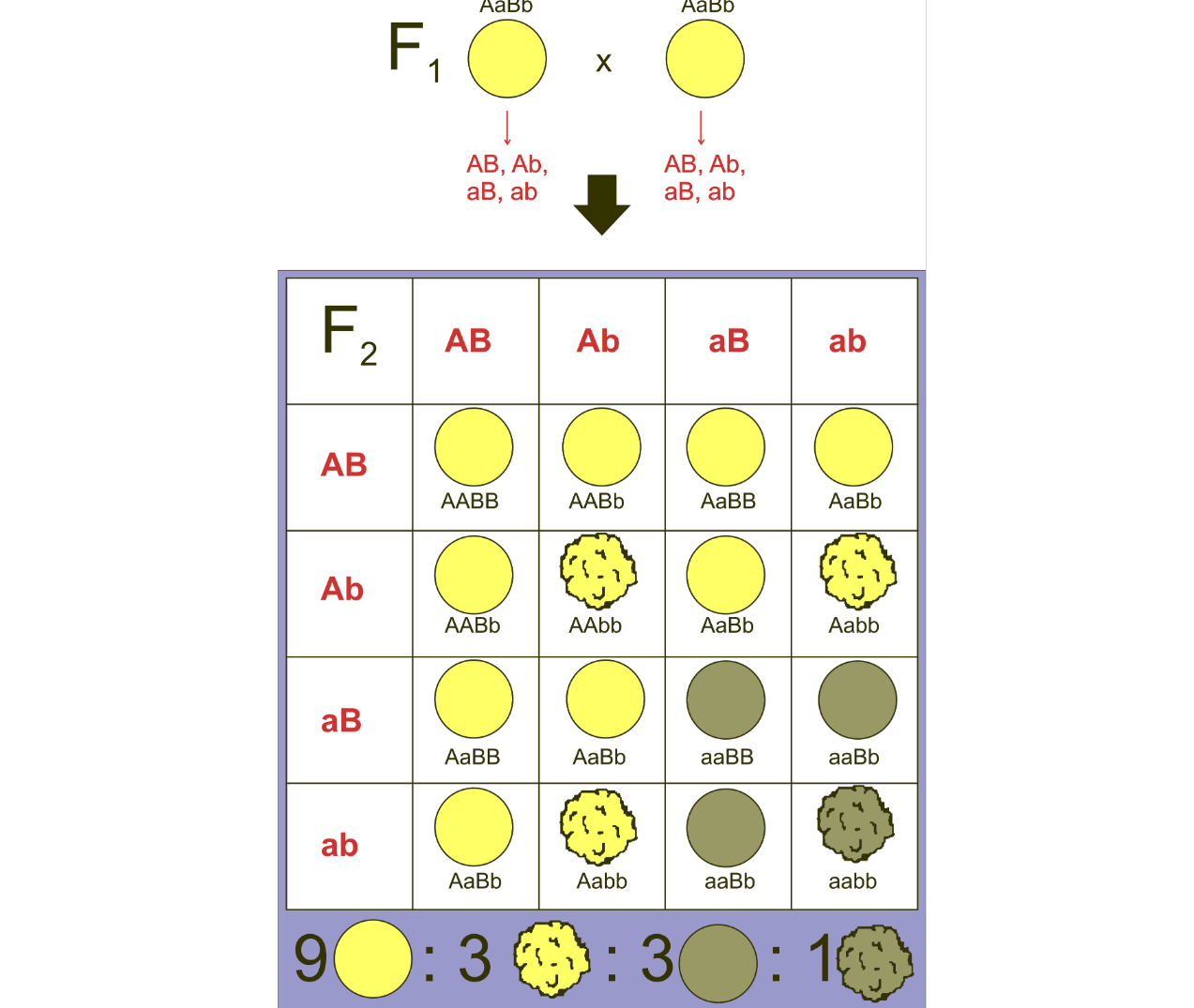
It is the case that both of Mendel’s laws works out if the two traits are each only controlled by one gene, and that the genes controlling these traits are on different chromosomes. Let us do an example. We have two types of peas, one which is yellow and round, and another one which is green and wrinkled. Mendel found out that yellow is dominant to green, and that round is dominant to wrinkled. He also only used pure breeding peas, which means that the peas were homozygous for the trait. The yellow round peas therefore had the genotype YYRR, and the green wrinkled peas, the genotype yyrr. It is important to note that the genes controlling color and round/wrinkled are on different chromosomes. When YYRR is crossed with yyrr, the only possible resulting genotype is YyRr because YYRR can only produce YR gametes, and yyrr can only produce yr gametes.
It gets more interesting when the YyRr peas are crossed with yyrr peas. Crossing back to a double homozygous recessive genotype is called a test cross because it tests whether genes are independent or not, which we will come back to later. The resulting Punnett square is also much easier to draw, since yyrr can only produce yr, it becomes a one by four Punnett square instead of a four by four Punnett square. The YyRr pea can produce gametes with YR, Yr, yR, or yr. The resulting genotypes are YyRr, Yyrr, yyRr, and yyrr.
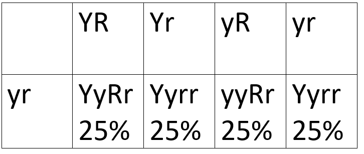
The genotypes themselves are not important, what is important is that they come in a 1:1:1:1 ratio. This means that they are all equally likely, so they follow Mendel’s first and second laws.
If we were to self-breed the YyRr peas, we would get the typical four by four Punnett square with a phenotype ratio of 9:3:3:1. In a 2 by 2 Punnett square with two heterozygote parents, we would get a 3:1 phenotype ratio.
Linked traits
Linked traits means that the genes for the traits lie on the same chromosome. The most famous experiment on linked traits (which was the experiment done to prove linked traits) was done on fruit flies. Fruit flies uses a special notation because the flies tested were either normal or mutant. Normal flies were yellow and had normal wings, while mutant flies were black and had vestigial wings (crunched up wings). The notation for normal color and wings is “+”, while the notation for black is “b” and vestigial wings is “vg”. When a purebred fly with normal color and normal wings (++,++) is bread with a purebred fly with a black body and vestigial wings (bb, vgvg), all of the offspring gets the genotype (b+, vg+). It turned out that the genotype b+,vg+ was a yellow fly with normal wings, which means that the normal coloring and wings were dominant (which makes sense, otherwise we would see a lot of walking flies). The problem arises when these flies are test bred back to the double homozygous recessive parent, because Mendel’s laws would predict a 1:1:1:1 ratio.
This did not turn out to be the case, because the probability of the recombinant genotypes was only 17%, which is not in accordance with Mendel’s laws. We now know that the reason for this is because the genes for color and type of wings is on the same chromosome, which means that the only way to get the recombinant allele, is for recombination to occur. Recombination can occur wherever on the chromosome, so genes far away from each other have a bigger chance of being recombined, and genes close to each other have a smaller chance of getting recombined. The percentage ratio of recombined genotyped therefore depend on the distance between the genes. In this experiment we got 17%, but if the genes were to be closed to each other, we would get a percentage lower than 17%, and if they were farther from each other, we would get a percentage greater than 17%. This is the reason why people with red hair tend to have freckles, because the genes are on the same chromosome. This is also the reason why test crossing is done, because if the ratio is 1:1:1:1, it means that the genes are on different alleles, but if the ratio is something else, it suggests that the genes are on the same chromosome.
This is normally very confusing, so I would recommend watching this video:
https://www.youtube.com/watch?v=-_UcDhzjOio
Chi squared tests are commonly used to see if there is a statistical correlation between the observed value and the expected value. For more information about chi squared tests, visit topic 4.
Hardy-Weinberg equation
A gene pool is the total sum of alleles in a population which an individual of that species can have. A big gene pool means more variation, while a small gene pool means less variation. Allele frequency is a percentage measurement in how many individuals in a population has one specific allele. For example, if we have a population of two individuals (not much of a population) and one has genotype Ff, and the other has FF. The allele frequency of f is then 1/4, and the allele frequency of F is 3/4. Notice that they always add up to 1, which is the basis of the Hardy-Weinberg equation. Let us call the frequency of the dominant allele for p, and the frequency of the recessive allele for q. It will then be true that p + q =1. Since we are diploid organisms we have two copies of each gene, so the equation becomes (p +q)2 = 1. Expanding the equation then gives us p2 + 2pq + q2 = 1, which is the Hardy-Weinberg equation. It basically shows the ratios between dominant homozygote, heterozygote, and homozygote recessive. Try to see how the equation relates to a Punnett square crossing two heterozygote individuals. This equation can solve problems for example involving allele frequencies and finding how many individuals of a population has a specific phenotype.
To see examples of problem-solving with the Hardy-Weinberg equation, watch this video:
https://www.youtube.com/watch?v=xPkOAnK20kw
Isolation, selection, and speciation
A number of factors can isolate a species into two or more groups, which results in two or more isolated gene pools. Isolated gene pools can speciate into new species with time, which was seen with adaptive radiation in topic 5. Geographical isolation is when physical barriers such as a mountain or a lake separates groups in a species so that they cannot mate anymore. Temporal isolation is when time separates species from mating. This could be fertility at different seasons, or different patterns of hibernation. Behavioral isolation is when behavior isolates two groups. This could be for example different mating rituals or diet.
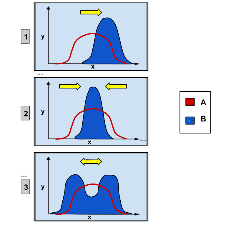
Selection patterns is how nature selects different phenotypes. Directional selection means that one phenotype is more favored than one other, and the frequency of the favored phenotype will increase as the frequency of the less favored phenotype decreases. This could for example be seen if a sharp beak is more favorable. There would be more and more sharp beaks, and less and less blunt beaks. Stabilizing selection is when nature selects for a median in between two extremes. For example, choosing a flower producing an intermediate amount of nectar instead of flowers producing too little or too much nectar. Disruptive selection is the opposite of stabilizing selection. In disruptive selection, the two extremes are selected instead of the intermediate. This could for example be if black or white color is favorable, but not black and white. It is possible for speciation to occur if the two extremes become so different that they can no longer breed fertile outcome.
1: directional selection 2: stabilizing selection 3: disruptive selection A: before B: after
There are two conflicting views of speciation. The first view says that speciation is a continuous gradual change in traits, while the other view says that the changes are abrupt and that a long period of no change follows the speciation. The first view is called gradualism, while the other is called punctuated equilibrium.
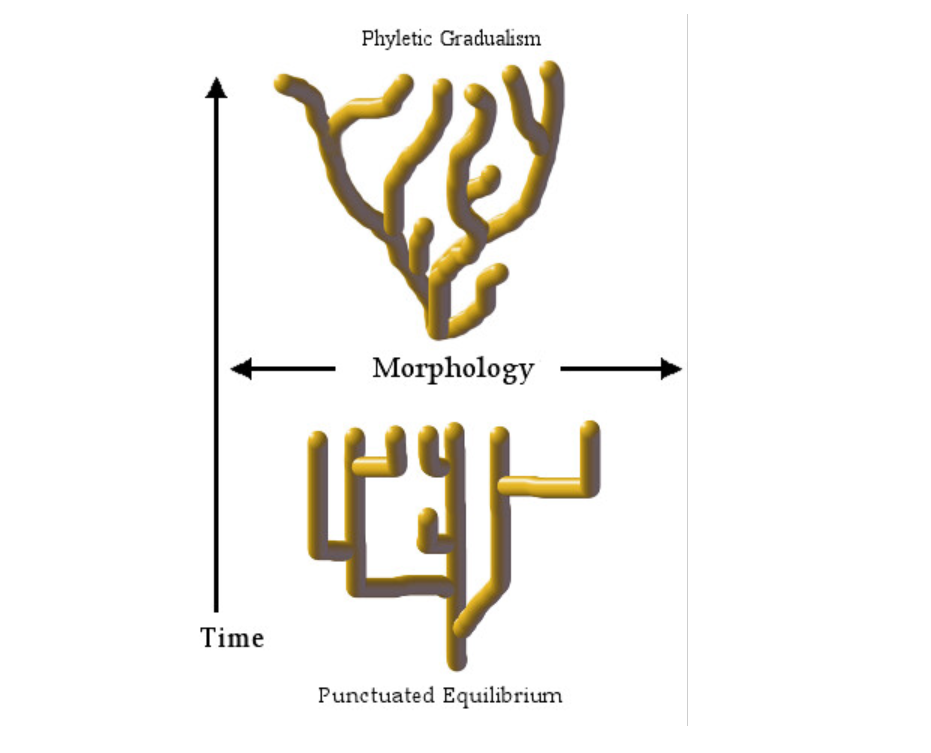
To read more about the different views on speciation, visit: https://necsi.edu/gradualism-and-punctuated-equilibrium
Helpful videos:
Meiosis: https://www.youtube.com/watch?v=16enC385R0w
Dihybrid Punnett squares: https://www.youtube.com/watch?v=Y1PCwxUDTl8
MIT series on Mendel’s laws part 1:
https://www.youtube.com/watch?v=9dHBTckFvME&list=LL&index=7
MIT series on Mendel’s laws part 2:
https://www.youtube.com/watch?v=CT9lYy6qSfg&list=LL&index=5
MIT series on linked genes and recombination:
https://www.youtube.com/watch?v=o_1dTvszV4Y&list=LL&index=7
Linked genes and recombination:
https://www.youtube.com/watch?v=-_UcDhzjOio
Dihybrid crossing:
https://www.youtube.com/watch?v=1_lTyzGTnho
Hardy-Weinberg problems: https://www.youtube.com/watch?v=xPkOAnK20kw
I usually enjoy genetics a lot, and this topic was no exception. After finishing this topic, I feel like I have a whole new perception of genetics and heredity. I found dihybrid crossing interesting because it answered question I did not even have, and I liked the Hardy-Weinberg equilibrium because it shows how math can suddenly appear from nowhere. Otherwise, I would highly recommend the linked videos from MIT because I understood so much from watching them.